Tidy Tuesday Exercise 2

Load in the code

tuesdata <- tt_load('2023-04-11')
--- Compiling #TidyTuesday Information for 2023-04-11 ----
--- There are 2 files available ---
--- Starting Download ---

    Downloading file 1 of 2: `egg-production.csv`
    Downloading file 2 of 2: `cage-free-percentages.csv`
--- Download complete ---
eggproduction <- tuesdata[["egg-production"]][, 1:5]  #remove source as it won't be helpful to us
cagefreepercentages <-tuesdata[["cage-free-percentages"]][, 1:3]

Data Exploration and Cleaning

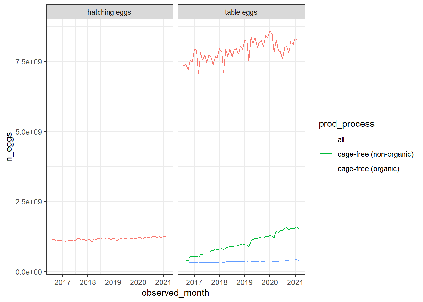
For the sake of this exercise, I’m going to be focusing on the eggproduction dataset. First I’m going to do some exploratory graphing to see what the general distributions look like. After looking, the structure of all the variables are as their supposed to be - dates as dates, numbers are numbers, etc.

ggplot()+
  geom_line(aes(x=observed_month, y= n_eggs, group=prod_process, color=prod_process), data=eggproduction)+
  facet_wrap(.~prod_type)+
  theme_bw()

This is great! This graph tells us a lot. First, it shows the data is pretty clean as the data graphed with no problems. It tells us that table eggs are produced at a vastly greater rate than hatching eggs, and that there are no cage-free hatched eggs. We also see a rise in production of table eggs for cage-free (nonorganic) and the total trend.

cor(eggproduction$n_hens, eggproduction$n_eggs)
[1] 0.9983136
ggplot()+
  geom_point(aes(x=eggproduction$n_hens, y= eggproduction$n_eggs, color=eggproduction$prod_process))

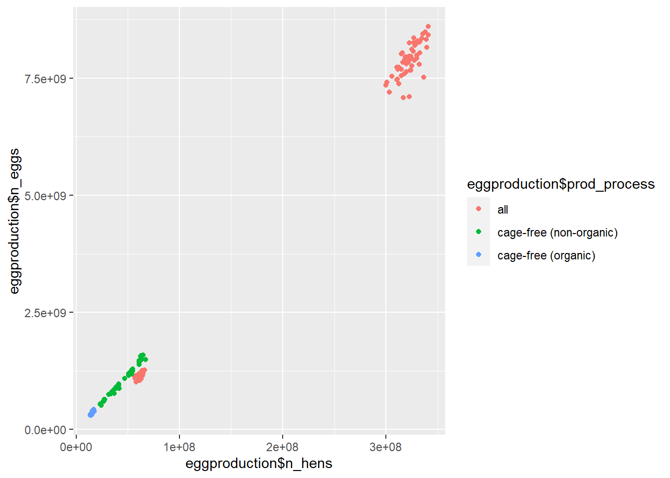
We see the differences in egg production by type of egg replicated in this scatter-plot, but we can also see the nearly straight correlation between the number of eggs and the number of hens across all groups. This doesn’t help us much in terms of creating a hypothesis about possible differences here.

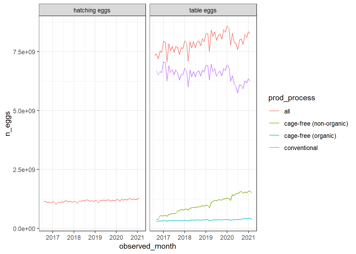
The only data cleaning I want to do off the bat is create another category rather than “all”, since this is a sum that includes cage-free and I want to see what the conventional housing distribution is alone.

eggproduction$n_eggs<-as.numeric(eggproduction$n_eggs)

egg_types<-spread(eggproduction, prod_process, n_eggs)%>%
  filter(prod_type == "table eggs", observed_month != "2016-07-31", observed_month != "2021-02-28")%>%
  select(-n_hens)%>%
  group_by(observed_month)%>%
  fill(`cage-free (organic)`, .direction = "down")%>%
  fill( all, .direction = "up")%>%
  fill(`cage-free (non-organic)`, .direction = "updown")%>%
  unique()%>%
  mutate(conventional = all -`cage-free (organic)`-`cage-free (non-organic)`)

Now that we have the calculated number of conventional egg production, we can merge back into our full dataset.

egg_types_tall<-gather(egg_types,key = prod_process, value = "n_eggs", all:conventional)

egg_types_all<-full_join(eggproduction, egg_types_tall)
Joining, by = c("observed_month", "prod_type", "prod_process", "n_eggs")

Graph it to make sure it worked

ggplot()+
  geom_line(aes(x=observed_month, y= n_eggs, group=prod_process, color=prod_process), data=egg_types_all)+
  facet_wrap(.~prod_type)+
  theme_bw()

Awesome! Now we can start looking into hypotheses and questions for our model.

Hypothesis Generation

While we have consistent information for trends related to years and within the number of eggs hatched per hen, I’m interested in seeing this data at the monthly level and within different production processes. To do this, I’m going to clean the data a bit further to focus on the table eggs since we have different production methods, elimininate the “all” option, and isolate the month the eggs were produced.

model_egg_data<-egg_types_all%>%
  filter(prod_type != "hatching eggs",
         prod_process != "all")%>%
  mutate(month = month(observed_month))%>%
  select(-observed_month, -n_hens, -prod_type)

model_egg_data$month<-as.factor(model_egg_data$month)

Based on the line graphs, it seems there dips in egg production around Feb/March each year. I predict that Feb/March has the greatest negative impact on egg production while early summer months (May/June) have the greatest positive impact on egg production. I’m using the production process as a strata in case this varies by process. Because of this, I am including the variable in the model.

Model Creation

Setting it Up

Split the data

set.seed(123)

data_split <- initial_split(model_egg_data, prop = 7/10, strata = prod_process) 

train_data <- training(data_split) 
test_data  <- testing(data_split)

We don’t a lot of entries for cross-validation due to only having 274 county/Food Bank combinations, so we’ll only do a 3x3 split.

folds <- vfold_cv(train_data, v = 3, repeats =3, strata = prod_process)

Create a recipe

egg_rates_recipe <- 
  recipe(n_eggs ~ ., data = train_data) %>%
  step_dummy(month, prod_process) 

Null Model

Build the model

null<-null_model() %>% 
  set_engine("parsnip") %>% 
  set_mode("regression") %>% 
  translate()

null_wf <-
  workflow() %>%
  add_model(null) %>%
  add_recipe(egg_rates_recipe)

null_fit <-
  null_wf %>%
  fit(train_data)

null_fit %>%
  extract_fit_parsnip() %>%
  tidy()
# A tibble: 1 × 1
        value
        <dbl>
1 2585493808.

View Trained RMSE

null_train_aug <- 
  augment(null_fit, train_data)

yardstick::rmse(null_train_aug, n_eggs, .pred)
# A tibble: 1 × 3
  .metric .estimator   .estimate
  <chr>   <chr>            <dbl>
1 rmse    standard   2764345202.

Test the Null Model

predict(null_fit, test_data)
# A tibble: 51 × 1
         .pred
         <dbl>
 1 2585493808.
 2 2585493808.
 3 2585493808.
 4 2585493808.
 5 2585493808.
 6 2585493808.
 7 2585493808.
 8 2585493808.
 9 2585493808.
10 2585493808.
# … with 41 more rows
null_test_aug <- 
  augment(null_fit, test_data)

yardstick::rmse(null_test_aug, n_eggs, .pred)
# A tibble: 1 × 3
  .metric .estimator   .estimate
  <chr>   <chr>            <dbl>
1 rmse    standard   2807740760.

Decision Tree

set.seed(123)

tune_spec <- 
  decision_tree(
    cost_complexity = tune(),
    tree_depth = tune()
  ) %>% 
  set_engine("rpart") %>% 
  set_mode("regression")

tree_grid <- grid_regular(cost_complexity(),
                          tree_depth(),
                          levels = 5)

tree_wf <- workflow() %>%
  add_model(tune_spec) %>%
  add_recipe(egg_rates_recipe)

tree_res <-
  tree_wf %>%
  tune_grid(
    resamples = folds, #recall this created CV from earlier
    grid = tree_grid)


tree_res %>%collect_metrics()
# A tibble: 50 × 8
   cost_complexity tree_depth .metric .estimator      mean     n std_err .config
             <dbl>      <int> <chr>   <chr>          <dbl> <int>   <dbl> <chr>  
 1    0.0000000001          1 rmse    standard     3.72e+8     9 8.48e+6 Prepro…
 2    0.0000000001          1 rsq     standard     9.83e-1     9 7.80e-4 Prepro…
 3    0.0000000178          1 rmse    standard     3.72e+8     9 8.48e+6 Prepro…
 4    0.0000000178          1 rsq     standard     9.83e-1     9 7.80e-4 Prepro…
 5    0.00000316            1 rmse    standard     3.72e+8     9 8.48e+6 Prepro…
 6    0.00000316            1 rsq     standard     9.83e-1     9 7.80e-4 Prepro…
 7    0.000562              1 rmse    standard     3.72e+8     9 8.48e+6 Prepro…
 8    0.000562              1 rsq     standard     9.83e-1     9 7.80e-4 Prepro…
 9    0.1                   1 rmse    standard     3.72e+8     9 8.48e+6 Prepro…
10    0.1                   1 rsq     standard     9.83e-1     9 7.80e-4 Prepro…
# … with 40 more rows
tree_res %>%
  show_best("rmse")
# A tibble: 5 × 8
  cost_complexity tree_depth .metric .estimator       mean     n std_err .config
            <dbl>      <int> <chr>   <chr>           <dbl> <int>   <dbl> <chr>  
1    0.0000000001          4 rmse    standard   269036936.     9  6.70e6 Prepro…
2    0.0000000178          4 rmse    standard   269036936.     9  6.70e6 Prepro…
3    0.00000316            4 rmse    standard   269036936.     9  6.70e6 Prepro…
4    0.000562              4 rmse    standard   269036936.     9  6.70e6 Prepro…
5    0.0000000001          8 rmse    standard   269036936.     9  6.70e6 Prepro…
best_tree <- tree_res %>%
  select_best("rmse")

best_tree
# A tibble: 1 × 3
  cost_complexity tree_depth .config              
            <dbl>      <int> <chr>                
1    0.0000000001          4 Preprocessor1_Model06
final_wf <- 
  tree_wf %>% 
  finalize_workflow(best_tree)

final_fit <- 
  final_wf %>%
  last_fit(data_split) 

final_fit %>%
  collect_metrics()
# A tibble: 2 × 4
  .metric .estimator     .estimate .config             
  <chr>   <chr>              <dbl> <chr>               
1 rmse    standard   271027592.    Preprocessor1_Model1
2 rsq     standard           0.991 Preprocessor1_Model1
final_fit %>%
  collect_predictions()
# A tibble: 51 × 5
   id                    .pred  .row      n_eggs .config             
   <chr>                 <dbl> <int>       <dbl> <chr>               
 1 train/test split 990191806.     1  397884291. Preprocessor1_Model1
 2 train/test split 990191806.     2  383774914. Preprocessor1_Model1
 3 train/test split 990191806.     6  550017411. Preprocessor1_Model1
 4 train/test split 990191806.    16  780750514. Preprocessor1_Model1
 5 train/test split 990191806.    18  826794977. Preprocessor1_Model1
 6 train/test split 990191806.    20  857017851. Preprocessor1_Model1
 7 train/test split 990191806.    23  882298286. Preprocessor1_Model1
 8 train/test split 990191806.    30  973820006. Preprocessor1_Model1
 9 train/test split 990191806.    32 1092870103. Preprocessor1_Model1
10 train/test split 990191806.    33 1147652743. Preprocessor1_Model1
# … with 41 more rows
final_tree <- extract_workflow(final_fit)
final_tree
══ Workflow [trained] ══════════════════════════════════════════════════════════
Preprocessor: Recipe
Model: decision_tree()

── Preprocessor ────────────────────────────────────────────────────────────────
1 Recipe Step

• step_dummy()

── Model ───────────────────────────────────────────────────────────────────────
n= 113 

node), split, n, deviance, yval
      * denotes terminal node

1) root 113 8.635013e+20 2585494000  
  2) prod_process_conventional< 0.5 76 1.166953e+19  673880700  
    4) prod_process_cage.free..organic.>=0.5 38 3.803180e+16  357569600 *
    5) prod_process_cage.free..organic.< 0.5 38 4.027492e+18  990191800 *
  3) prod_process_conventional>=0.5 37 3.647328e+18 6512050000 *
final_tree %>% 
  extract_fit_parsnip() %>% 
  vip()

LASSO

For the lasso I’m changing up the workflow based on a resource a classmate recommended to me by one of the tidymodels creators. We’re going to see if I have better luck with these methods. Her explanations were very helpful, and hopefully her methods will work on my data!

TRAIN

##TRAIN
lr_mod <- linear_reg(penalty = 0.1 , mixture = 1) %>% 
  set_engine("glmnet")

lr_workflow <- 
  workflow() %>% 
  add_recipe(egg_rates_recipe)

lasso_fit<- lr_workflow%>%
  add_model(lr_mod) %>% 
  fit(data = train_data)

lasso_fit%>%pull_workflow_fit()%>%tidy()
Warning: `pull_workflow_fit()` was deprecated in workflows 0.2.3.
ℹ Please use `extract_fit_parsnip()` instead.
Loading required package: Matrix

Attaching package: 'Matrix'
The following objects are masked from 'package:tidyr':

    expand, pack, unpack
Loaded glmnet 4.1-6
# A tibble: 14 × 3
   term                                estimate penalty
   <chr>                                  <dbl>   <dbl>
 1 (Intercept)                      1052429681.     0.1
 2 month_X2                         -233101411.     0.1
 3 month_X3                           52030050.     0.1
 4 month_X4                          -68515442.     0.1
 5 month_X5                          -47909120.     0.1
 6 month_X6                         -102490754.     0.1
 7 month_X7                         -139746745.     0.1
 8 month_X8                          -61579946.     0.1
 9 month_X9                          -85382137.     0.1
10 month_X10                                 0      0.1
11 month_X11                         -19798883.     0.1
12 month_X12                                 0      0.1
13 prod_process_cage.free..organic. -638233204.     0.1
14 prod_process_conventional        5512551456.     0.1

TUNE

## TUNE
set.seed(123)

egg_boot <- bootstraps(train_data, strata = prod_process)

tune_spec <- linear_reg(penalty = tune(), mixture = 1) %>% 
  set_engine("glmnet")

lambda_grid<-grid_regular(penalty(),
             levels = 50)

set.seed(2023)
lasso_grid<- tune_grid(
  lr_workflow %>% add_model(tune_spec),
  resamples = egg_boot,
  grid = lambda_grid) #for each resample, trains the model

lasso_grid%>%
  collect_metrics()%>%
  ggplot(aes(x=penalty, y=mean, color = .metric)) + 
  # geom_errorbar(aes(ymin = mean - std_err, 
  #            ymax = mean + std_err),  alpha = 0.5 ) +
  geom_line(show.legend = F)+
  facet_wrap(.~.metric, scales = "free")

lowest_rmse<-lasso_grid %>% 
  select_best("rmse", maximize = F) # lowest rmse not highest 
Warning: The `maximize` argument is no longer needed. This value was ignored.
# shows penalty

final_lasso <- finalize_workflow(lr_workflow %>% add_model(tune_spec),
                  lowest_rmse) #is a workflow

FIT

#FIT IT
final_lasso%>%
  fit(train_data) %>%
  pull_workflow_fit() %>% 
  vi(lambda = lowest_rmse$penalty) %>%
  ggplot(aes(x=Importance, y=Variable, fill = Sign)) + 
  geom_col()

#for each variable in model, shows importance based on the lowest penalty in the workflow

TEST

# TEST 
last_fit(final_lasso, 
         data_split) %>%
  collect_metrics()
# A tibble: 2 × 4
  .metric .estimator     .estimate .config             
  <chr>   <chr>              <dbl> <chr>               
1 rmse    standard   285375418.    Preprocessor1_Model1
2 rsq     standard           0.990 Preprocessor1_Model1

Random Forest

cores <- parallel::detectCores()
cores
[1] 4
rf_mod <- 
  rand_forest(mtry = tune(), min_n = tune(), trees = 1000) %>% 
  set_engine("ranger", num.threads = cores) %>% 
  set_mode("regression")

rf_workflow <- 
  workflow() %>% 
  add_model(rf_mod) %>% 
  add_recipe(egg_rates_recipe)

set.seed(123)
rf_res <- 
  rf_workflow %>% 
  tune_grid(folds,
            grid = 4,
            control = control_grid(save_pred = TRUE),
            metrics = metric_set(rmse))
i Creating pre-processing data to finalize unknown parameter: mtry
rf_res %>% 
  show_best(metric = "rmse")
# A tibble: 4 × 8
   mtry min_n .metric .estimator        mean     n   std_err .config            
  <int> <int> <chr>   <chr>            <dbl> <int>     <dbl> <chr>              
1    10    36 rmse    standard    271931817.     9  8134330. Preprocessor1_Mode…
2     8    20 rmse    standard    305683208.     9 11762840. Preprocessor1_Mode…
3     4    10 rmse    standard    562228549.     9 20818240. Preprocessor1_Mode…
4     2    22 rmse    standard   1211747484.     9 13835416. Preprocessor1_Mode…
autoplot(rf_res)

rf_best <- 
  rf_res %>% 
  select_best(metric = "rmse")
rf_best
# A tibble: 1 × 3
   mtry min_n .config             
  <int> <int> <chr>               
1    10    36 Preprocessor1_Model2
rf_res %>% 
  collect_predictions()
# A tibble: 1,356 × 8
   id      id2         .pred  .row  mtry min_n      n_eggs .config             
   <chr>   <chr>       <dbl> <int> <int> <int>       <dbl> <chr>               
 1 Repeat1 Fold1 1171372315.     1     8    20  546374469. Preprocessor1_Model1
 2 Repeat1 Fold1  944487209.     9     8    20  643637057. Preprocessor1_Model1
 3 Repeat1 Fold1 1171372315.    12     8    20  804085971. Preprocessor1_Model1
 4 Repeat1 Fold1  944487209.    17     8    20  908679086. Preprocessor1_Model1
 5 Repeat1 Fold1 1171372315.    20     8    20  967391846. Preprocessor1_Model1
 6 Repeat1 Fold1 1194774866.    25     8    20 1170483943. Preprocessor1_Model1
 7 Repeat1 Fold1  867253524.    28     8    20 1248814800  Preprocessor1_Model1
 8 Repeat1 Fold1  909115772.    29     8    20 1290441960  Preprocessor1_Model1
 9 Repeat1 Fold1  929376494.    30     8    20 1271439669. Preprocessor1_Model1
10 Repeat1 Fold1  918020490.    31     8    20 1189411303. Preprocessor1_Model1
# … with 1,346 more rows
rf_rmse <- 
  rf_res %>% 
  collect_predictions(parameters = rf_best) 
rf_rmse
# A tibble: 339 × 8
   id      id2         .pred  .row  mtry min_n      n_eggs .config             
   <chr>   <chr>       <dbl> <int> <int> <int>       <dbl> <chr>               
 1 Repeat1 Fold1  957482614.     1    10    36  546374469. Preprocessor1_Model2
 2 Repeat1 Fold1  937284386.     9    10    36  643637057. Preprocessor1_Model2
 3 Repeat1 Fold1  957482614.    12    10    36  804085971. Preprocessor1_Model2
 4 Repeat1 Fold1  937284386.    17    10    36  908679086. Preprocessor1_Model2
 5 Repeat1 Fold1  957482614.    20    10    36  967391846. Preprocessor1_Model2
 6 Repeat1 Fold1 1009461459.    25    10    36 1170483943. Preprocessor1_Model2
 7 Repeat1 Fold1  932026806.    28    10    36 1248814800  Preprocessor1_Model2
 8 Repeat1 Fold1  945577696.    29    10    36 1290441960  Preprocessor1_Model2
 9 Repeat1 Fold1  941033723.    30    10    36 1271439669. Preprocessor1_Model2
10 Repeat1 Fold1  953236486.    31    10    36 1189411303. Preprocessor1_Model2
# … with 329 more rows

Model Evaluation

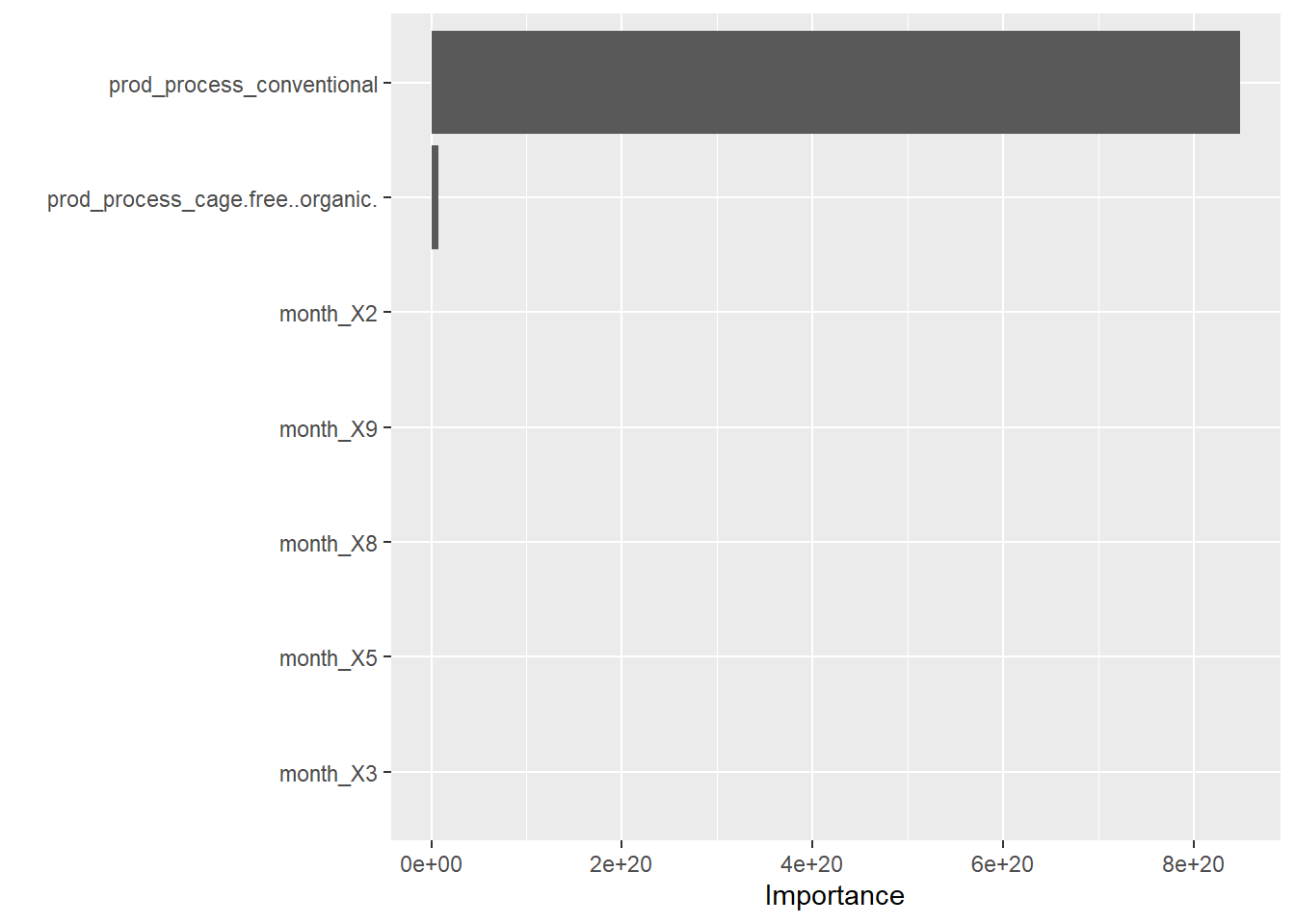
There are several obvious drawbacks to these methods. I was trying to determine the month with the largest impact on egg production, controlled for egg production type. However, the tidymodels framework did not allow for this or eliminating the variable to only include month. Therefore, since conventional production was such a large percentage of the eggs produced, it was often included in the model. This was especially evidenced in the decision tree. Therefore, this scored the most poorly of all the models since it could not discern any other variations within the data.

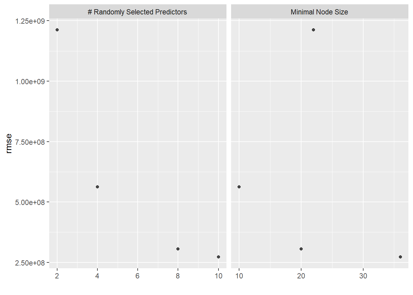
Next, and I think this is user error, is I’m not sure how to pull out the significant predictors for random forest models. I’m not sure if I’m overlooking a basic command or if this is so much of a “black box” model that we just have to take it at its word. For this reason, I would not choose to use a model.

Then, we have the null model. It’s great for averages, but does not give us good change over time, and its RMSE was insanely high for both the trained and tested data. But it’s an average, which can’t go too wrong, just not very powerful for answering questions about the data itself.

That leaves the LASSO model. I switched workflows to mirror one from a tidymodels creator, and it was very helpful and intuitive to what the steps in the code were doing. I’m not sure if these can be applied to other model types because by the end of this exercise workflows, parameters, and grids were swimming too much in my head to identify the exact differences in coding styles and apply it to the other model types.

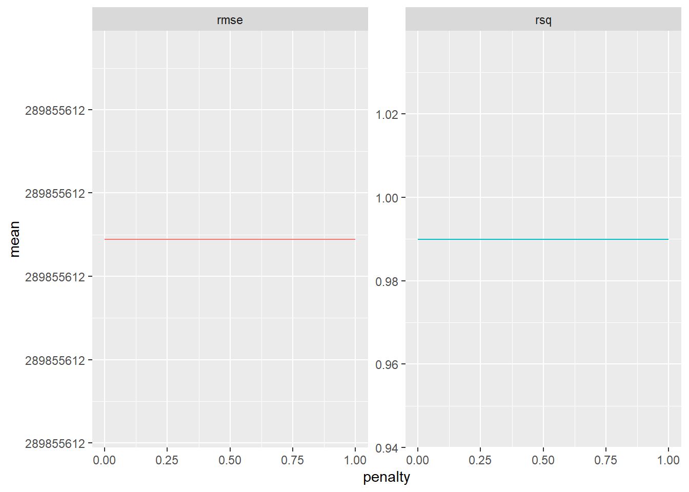
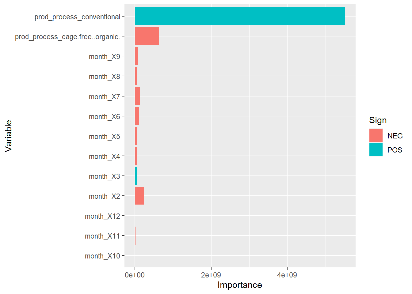
I really liked being able to see the importance of the factors using the graph in the final fit. As predicted, February had a very strong negative effect on egg production, while March actually had a positive impact on egg production - likely a strong bounce-back after the dip in February. I wonder again if the strong impact of production type overshadows the true impact other months have, as I doubt that all months truly have a negative impact on egg production since the general trend of egg production overtime was increased. However, I’m not sure how effective these models actually are since the visual of RMSE/RSQ were straight lines. Again, I don’t know if it’s the model, or how I coded it which actually created the error.

Overall, this exercise helped strengthen my understanding of tidymodels, but I still have a long way to go, especially with tree-based designs and truly comprehending how this framework works to adapt to different data.